Project Blog
Authors: Pratim Ugale, Yifan Zhang
Code: https://github.com/pratimugale/cisc662
As part of a graduate Computer Architecture course project that we were taking last semester, we set out to explore how Quantum Computing simulations are performed on GPUs. This blog details out the work that was done during the project, the library and GPU profiling software used, and the results.
An Introduction to Quantum Computing
Quantum computation is a paradigm of computing that utilizes the behaviour of quantum mechanics. While we do not get into the details of the way quantum computing works in this post, the key points to highlight are:
Similar to classical computers in which gates act on bits to do computation, quantum computers have quantum gates that operate on qubits. Quantum gates have matrix representations, where the matrix is Unitary. This matrix acts on a state vector that represents the state of the qubits. A qubit can exist in a superposition of 0 and 1 and a state. Two qubits can exist in a superposition of 00, 01, 10, and 11, and similarly n qubits can exist in 2n computational basis states. Each of these basis states (for eg. 01 in 2 qubit case) has a probability amplitude associated with it, and the square of the magnitude of this complex number yields the probability of the n-qubit system being in this state.
The state of the quantum system is hence represented by a state vector of size 2n, each element of which is a complex number. When a quantum gate (2n x 2n unitary matrix of complex numbers) is applied to a state vector, the resultant state vector gives the new probability amplitudes of the states, and thus the new probabilities of measurement. New gates would in turn modify this resultant vector and the matrix-vector multiplications form the basis of parallelization using GPUs.
To make the comparisons useful, we perform simulations on one of the recent quantum algorithms - the Quantum Approximate Optimization Algorithm (QAOA) [1]. Following are the key concepts of QAOA: (To see a detailed explanation, please see another blog I have written here)
- QAOA is used to solve Combinatorial Optimization problems which involve finding an optimal element (solution) from a finite set of elements, such that an objective function is maximized or minimized. For example, the MaxCut problem is a Combinatorial Optimization problem - it involves splitting the vertices of a graph into two sets such that the number of edges between the two sets of vertices is maximized. We use QAOA to solve for MaxCut in our experiments.
- QAOA is an approximate algorithm - It involves applying two kinds of parameterized gates alternatively for a repeated number of times.
One set of two gates is called a “layer” of QAOA. The more the number of layers that one uses, the better the approximation gets [1]. A problem graph is represented by a Hamiltonian whose highest value eigenstate corresponds to the optimal solution. Also, one needs to find good parameters as the circuit contains parameterized gates, and a good solution is obtained after finding good parameters. This process involves starting with some initial parameters, finding the expectation value of the resultant state according to a known Hamiltonian and then optimizing the parameters until the expectation value is maximized. This process can utilize different kinds of optimizers - like COBYLA (Constrained Optimization by Linear Approximation), NelderMead, and others.
Implementation
To start implementing the project, we started looking for libraries that provide APIs for applying gates on GPUs and very quickly found out about CUDA-Q (CUDA-Quantum: https://developer.nvidia.com/cuda-q) which supports programming quantum computers using an API that can use various QPUs (Quantum Processing Units) as backends and also supports simulations on GPUs and CPUs.
CUDA-Q provides various examples and programs from simple quantum gates to more advanced algorithms like the Variational Quantum Eigensolver and QAOA. We use this example of QAOA, and extend it to take bipartite graphs as inputs so that it becomes easier to verify the solution. A bipartite graph is already partitioned into two sets, hence we can verify if the solution is correct by checking if the algorithm correctly assigned all the vertices to the correct set. Our Professor, Dr. Sunita Chandrasekaran provided us access to the GPUs on Bridges-2 and Delta Supercomputers. We also extend the code to make it easier to perform various and extensive experiments when using it with SLURM jobs. For example, the program requires 4 parameters:
Number of nodes to solve for - this also is equal to the number of qubits being simulated, because for MaxCut, QAOA requires the number of qubits equal to the number of nodes in the graph.
Number of layers - increasing this gets us a better solution. However when using GPUs the number of computations required increase and in case of a quantum processor, the depth of the circuit increases.
Optimizers - We use COBYLA in the results presented here. We also tried out NelderMead when performing some experiments.
Target - Can be set to various targets that CUDA-Q provides - like CPU (target=qpp-cpu) or GPU (target=nvidia)
We can thus design SLURM job batch scripts which can iterate over various parameters, and execute the simulation for a given node size and layer size. We collect various metrics like:
Total time required to execute the program
Time required for optimization
Time required for sampling the solution (measurement)
Time taken for finding the solution that was sampled for the maximum amount of times
The max cut found out by the algorithm after the optimization was complete
For some programs, other profiling data, obtained from the Nvidia Nsight Compute Profiler (ncu). This was done only for some programs as profiling takes relatively a very large amount of time and does not accurately reflect the actual time the program takes.
Installing CUDA-Quantum and Nsight Compute on the two supercomputers:
We start with looking for modules on Bridges-2 that contain CUDA-Quantum. We were not able to find a module, but could see a Singularity image that had CUDA-Quantum version 0.7.0 installed. This seems like an excellent place to start with, as Singularity allows reproducing the exact same environment on different supercomputers without requiring root privileges to run the containers (unlike docker). We start using this image to set up initial experiments - we note the time it takes for some parameters but soon realize that we cannot use the Nsight Compute binary directly that comes installed in the host with the “cuda” module. To solve this, we install Nsight Compute CLI (ncu) on top of the Singularity image. We do this by writing a Singularity definition file, which is similar to a Dockerfile which is used for creating Docker images. We take the latest CUDA-Q docker image (nvcr.io/nvidia/nightly/cuda-quantum) tagged cu11-latest and add a postscript to update the GPG repository keys and install ncu using apt - see Apptainerfile.def. The references for this process can be found here: https://developer.nvidia.com/blog/updating-the-cuda-linux-gpg-repository-key/ and https://nvidia.github.io/cuda-quantum/latest/using/install/local_installation.html#singularity. We install the 2024.3.2 version of Nsight Compute, use the command singularity build --fakeroot cudaq-env.sif Apptainerfile.def to locally build the image on our laptop, which we then transfer to the remote computer. With this, the setup is now complete.
Results
We run our experiments on the following:
- V100 GPU that is available on Bridges-2 and has 32GB of memory.
- A100 GPU that is available on Delta and has 40GB of memory.
- CPU of Bridges-2 that has the Intel Xeon Gold 6248 processor.
We find out that the optimization time usually dominates and takes up the bulk of the time required for the program. We first set to plot the optimization time against the number of nodes in the bipartite graph and obtained the following plot:
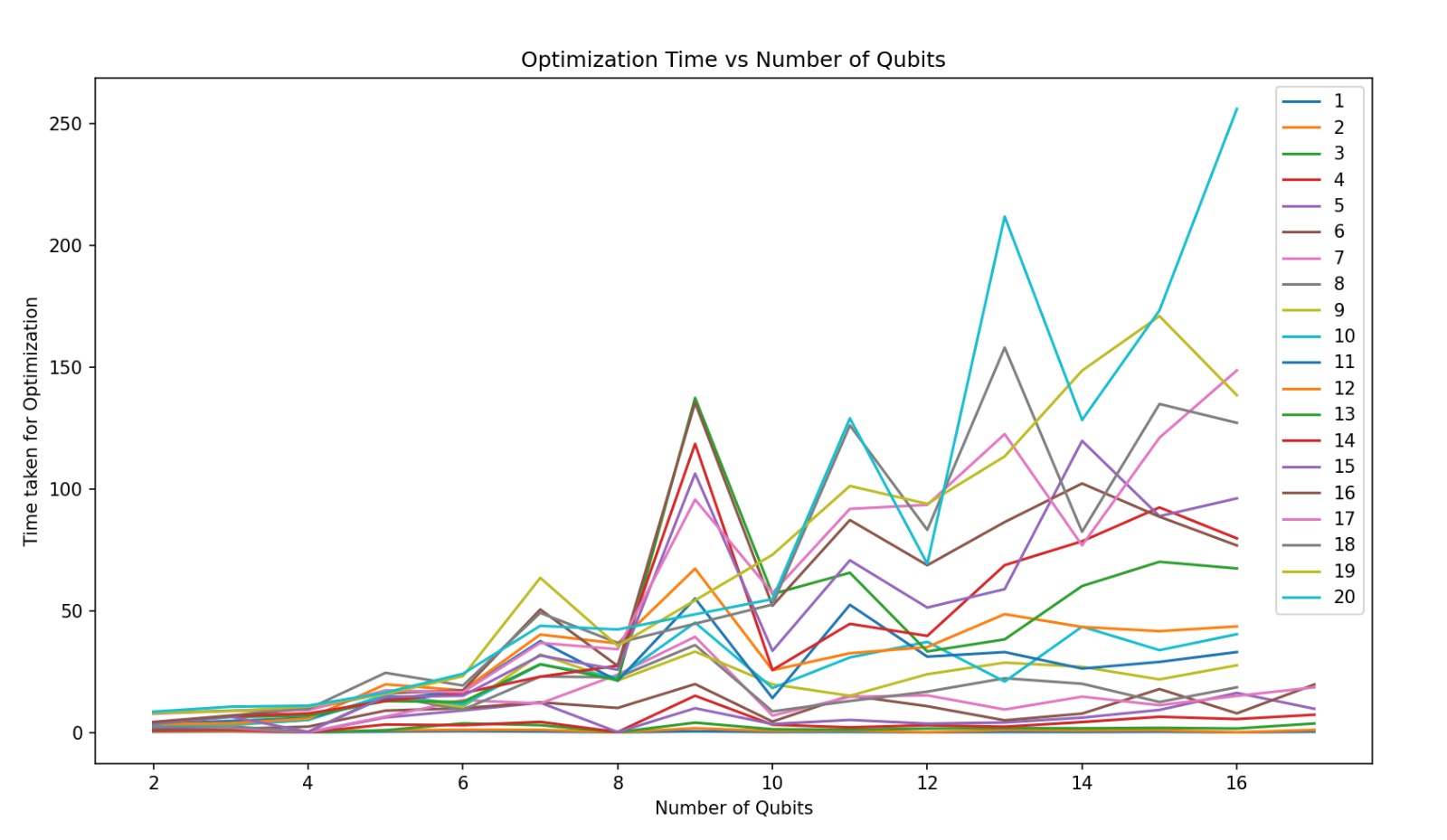 The unit of time here is seconds. We can see that the time required for the optimization to complete does not uniformly increase, as expected because the state vector size doubles for every increase of 1 qubit. We also noticed that a lot of the times, the actual MaxCut result obtained were not accurate.
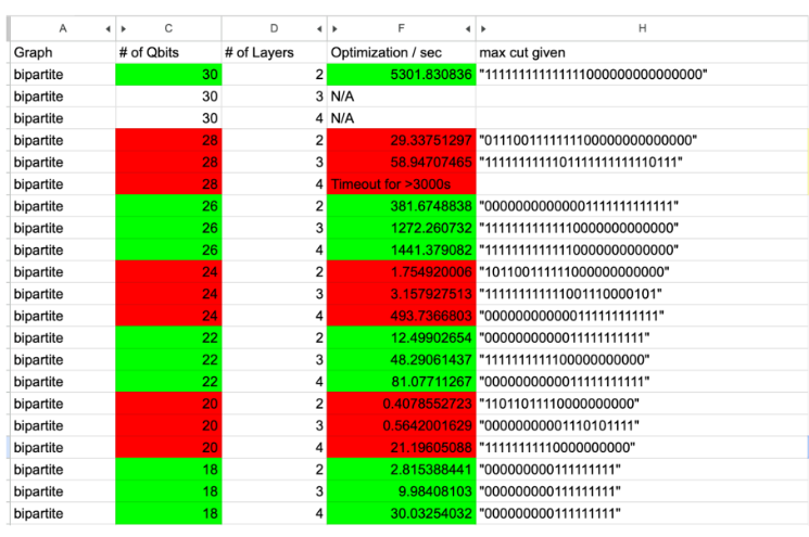
Identifying the cause of this issue took us quite some time as it could have multiple reasons - our understanding of the algorithm, the optimizer being used, or perhaps because it could be a characteristic of the graph structures we were using because testing only on bipartite graphs could be a special case. We dived deeper to check why it happens. On using a different optimizer, NelderMead, we obtained a bit better results in terms of cut values for larger number of qubits, but the optimization times still varied similar to the plot above (increasing qubits could give smaller optimization time). Following is the Time (s) vs Number of Qubits plot when using the NelderMead optimizer:
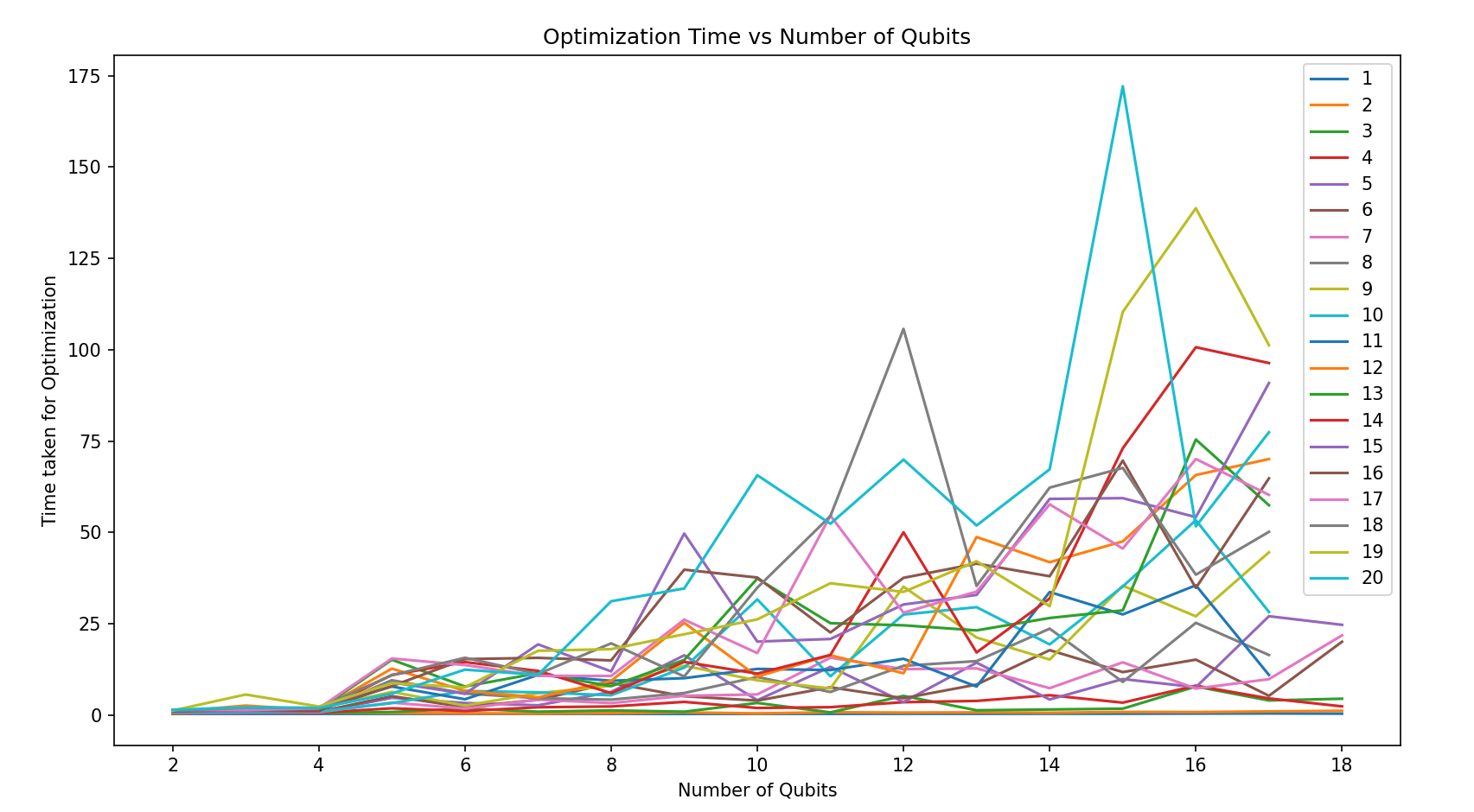
We can see that this has a fluctuating time required for optimization as well without any obvious pattern.
By tweaking the parameters of the optimizer, it eventually turned out that the cause of the fluctuating optimization time was the number iterations that the optimizer took to converge. On setting a limit on the maximum number of iterations to 100, we found out that not only does the optimization time become more predictable, but also the accuracy of the results improve significantly even for larger number of qubits. Following is the new plot of Time vs Number of Qubits/Nodes:
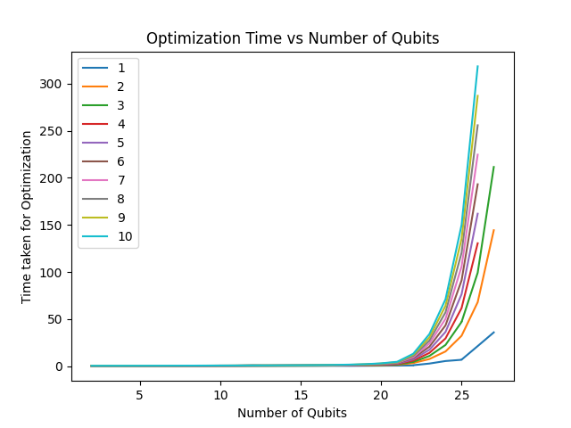
The reason why the stopping criteria was taking lesser time for a bigger graph in some cases is something that is left out of the scope of this project. To understand more about why more iterations gave worse results for COBYLA, I am planning to understand better how derivative-free optimizations work, and plan write another blog detailing this. The work has been started here, more to follow!
Once this was done, we now had a stable code that was providing consistent time for optimization and at the same time was accurate. We thus moved to comparing the optimization time against cpu (on Bridges-2), V-100 GPUs (on Bridges-2) and A-100 GPUs (on Delta). Following is the plot obtained for increasing number of qubits vs optimization time in seconds, for 1 layer of QAOA.
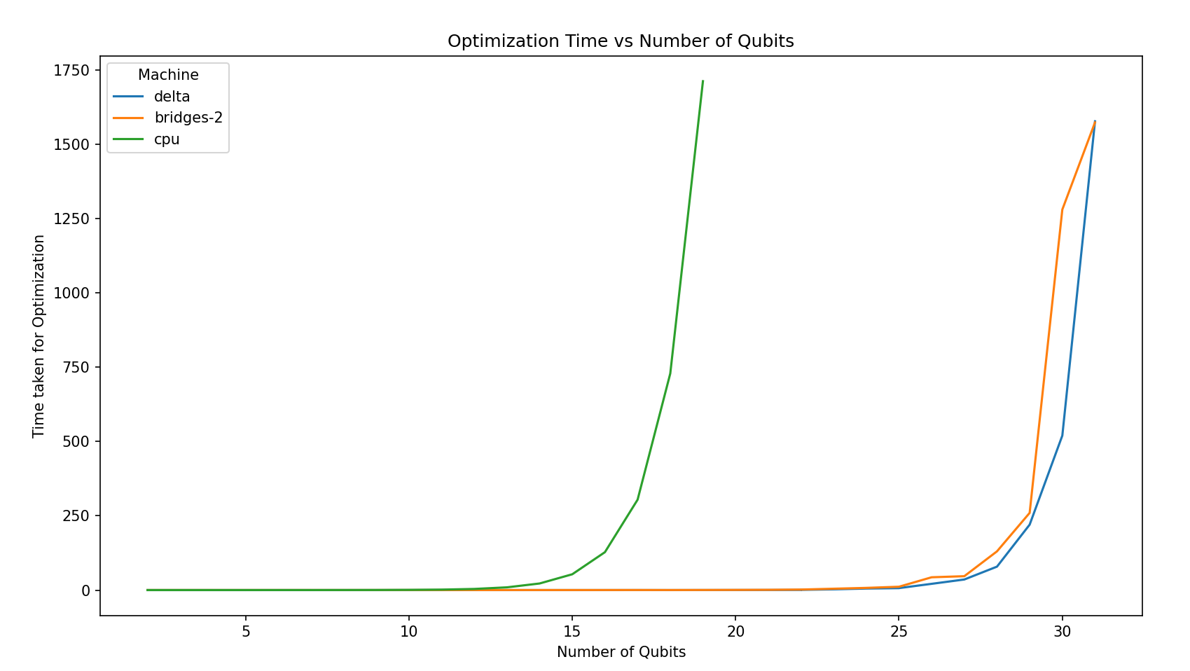
We can see that at 19 qubits and 1 layer for the cpu (Bridges-2), the runtime already reaches 1712.128s and time taken is slightly over double after 10 qubits. 19 qubits is the maximum number of qubits we could simulate. Similarly 31 qubits is the maximum that we could simulate for a Bridges-2 (V-100 SXM) GPU. The performance of Delta in terms of time is slightly better than Bridges-2 but practically both scale in a similar manner.
On running the ncu profiler for 31 qubits on Bridges-2, we see the following metrics for the 1st kernel - cudaInitializeDeviceStateVector which initializes the qubits to a \(\\|000...0>\) state, which is used as a start state for many algorithms. Following is the Speed of Light (SOL) plot:

We can clearly see that this kernel is memory bound and is utilizing almost all of the available memory bandwidth (99.98% or 898.26 Gbyte/s) where the max is 900 GB/sec for a V-100 SXM GPU (source: https://images.nvidia.com/content/technologies/volta/pdf/volta-v100-datasheet-update-us-1165301-r5.pdf).
The grid dimensions of this kernel (cudaInitializeDeviceStateVector) is (8388608, 1, 1) x (256, 1, 1). 8388608 * 256 = 2147483648 = 231 for 31 qubits.
This falls in line to what one can expect, because each element of the state vector is a complex number having having two floating point numbers. By default, CUDA-Q uses precision of fp32.
Thus the memory used for just initializing the
state vector is 2 (floating point numbers) X 231 (size of state vector) X 32 bits (size of variable - fp32) = 16 GB.
On increasing the number of nodes (and thus qubits) to 32, we see the following error thrown by CUDA-Q:
RuntimeError: NLOpt runtime error: nlopt failure
One can expect this as well because the memory required would be 32 GB. We set the log-level of CUDA-Q to info to give us more info about what is going on underneath and are able to validate our reasoning with the following:

We can see that we are not able to even allocate a new state vector for 32 qubits.
Following is the memory chart for 31 qubits for which the SOL plot is shown above:
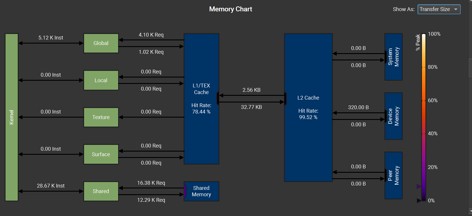
The theoretical occupancy for this kernel was 100% and the achieved occupancy was 82.08%

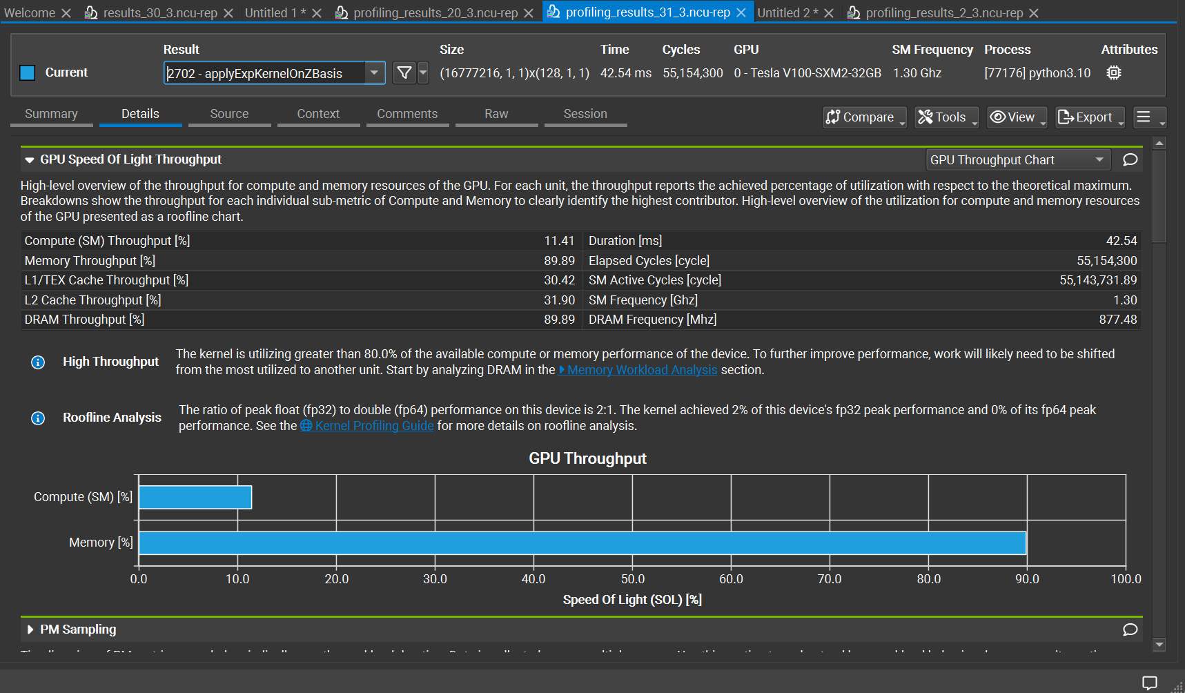
On checking other kernels of this program, we still see from the Speed of Light Throughput plots that the kernel utilizes more of the memory throughput as compared to the compute throughput, as seen in one of the other kernel’s (applyExpKernelOnZBasis) plot below:
Another analysis that we wanted to do was - for a fixed number of nodes, how does the time required for optimization (max 100 iterations) scale with the number of layers used in QAOA. This is because more layers are usually beneficial and usually dont do worse than less number of layers in QAOA[1]. We get the following plot and can see that the time required increases almost linearly upto 10 layers for 31 qubits. Each line represents a fixed number of qubits, and this plot used data from simulations on a Delta GPU.
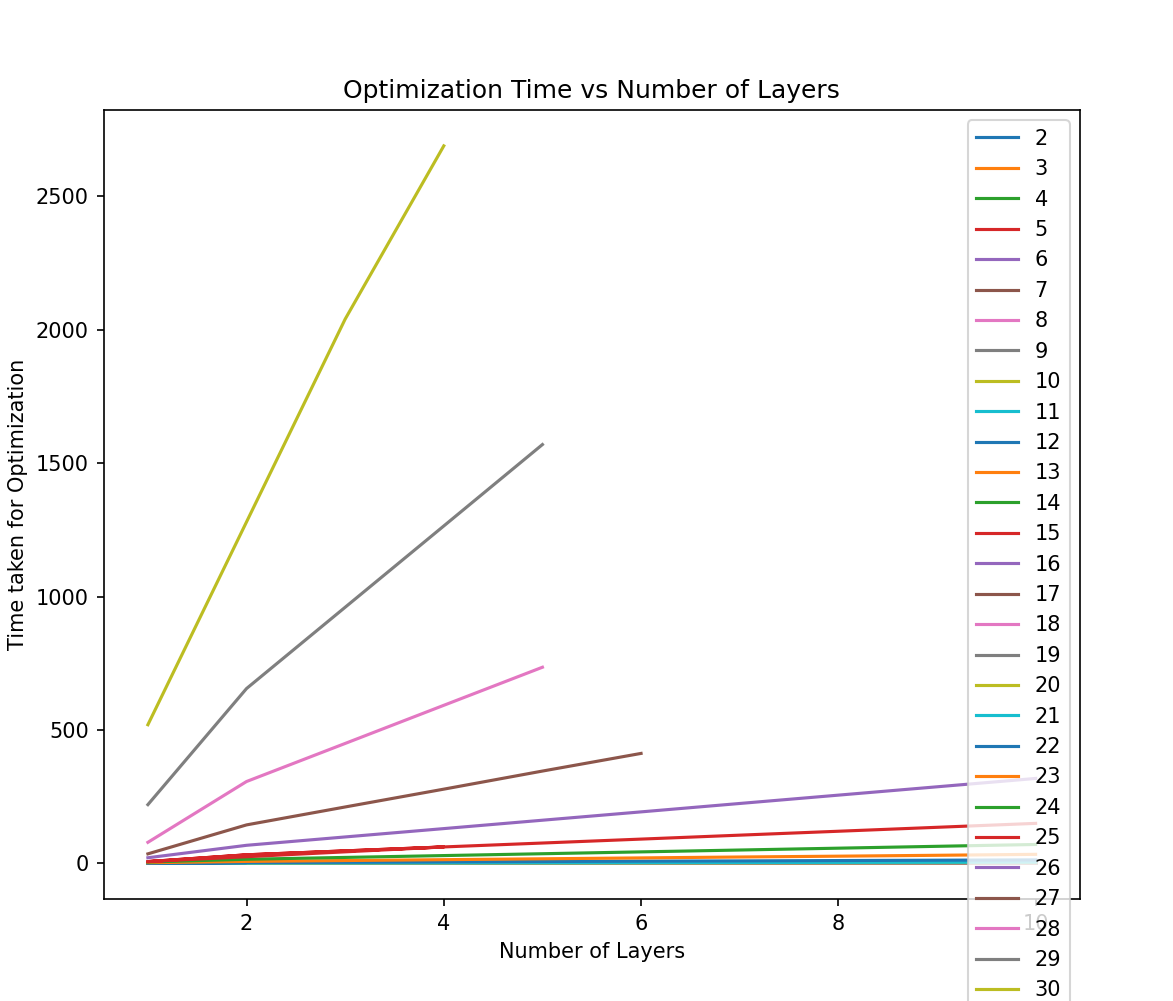
Using this, one can expect how the time required can grow for simulations on a GPU if more accurate results are required. One point to note is that this was done on a bipartite graph to ensure that the output was correct, and we still need to check the time on a more general graph.
Key Takeaways
Some topics of quantum computation were new to us, and through Nvidia’s examples we learned how algorithms like the Quantum Approximate Optimization Algorithm are implemented practically. We further run extensive experiments to see how one can leverage GPUs to perform simulations of algorithms up to 31 qubits, and how they scale with increasing layers. Any comments or feedback are most welcome!
To understand more about why more iterations gave worse results for COBYLA, I am planning to understand better how derivative-free optimizations work, and plan write another blog detailing this. The work has been started here, more to follow!
Acknowledgement
This work used Bridges-2 at Pittsburgh Supercomputing Center through allocation from the Advanced Cyberinfrastructure Coordination Ecosystem: Services & Support (ACCESS) program, which is supported by National Science Foundation grants #2138259, #2138286, #2138307, #2137603, and #2138296.
This research used the Delta advanced computing and data resource which is supported by the National Science Foundation (award OAC 2005572) and the State of Illinois. Delta is a joint effort of the University of Illinois Urbana-Champaign and its National Center for Supercomputing Applications.
This experiment builds upon the QAOA examples mentioned in the Nvidia CUDA-Quantum documentation: https://nvidia.github.io/cuda-quantum/0.8.0/using/examples/qaoa.html
References
[1] Edward Farhi, Jeffrey Goldstone, and Sam Gutmann. “A quantum approximate optimization algorithm”. In: arXiv preprint arXiv:1411.4028 (2014).
[2] https://nvidia.github.io/cuda-quantum/latest/index.html
[3] https://www.psc.edu/resources/bridges-2/user-guide/
[4] https://docs.ncsa.illinois.edu/systems/delta/en/latest/